0%

在神经网络中预测识别和预测的过程中,其实都是一个函数的对应关系: 的函数关系,为了找到这个函数的关系,我们需要做大量的训练,具体的过程可以总结下面几个步骤:

  1. 获得随机矩阵w1b1,经过一个激活函数,得到隐藏层。

  2. 获得随机矩阵w2b2,计算出对应的预测y

  3. 利用y与样本y_的差距,有平方差和交叉熵等方式,来定义损失函数

  4. 利用指数衰减学习率,计算出学习率

  5. 用滑动平均计算输出的参数的平均值

  6. 利用梯度下降的方法,减少损失函数的差距

  7. 用with结构初始化所有的参数

  8. 利用for循环喂入数据,反复训练模型

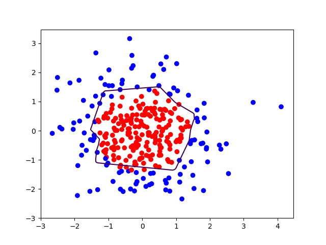
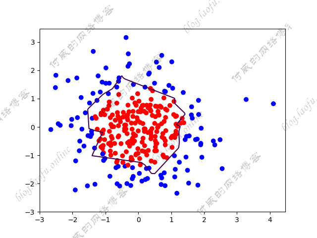
    利用这个八个步骤拟合出的一个圆的函数,代码和结果如下:

    1
    2
    3
    4
    5
    6
    7
    8
    9
    10
    11
    12
    13
    14
    15
    16
    17
    18
    19
    20
    21
    22
    23
    24
    25
    26
    27
    28
    29
    30
    31
    32
    33
    34
    35
    36
    37
    38
    39
    40
    41
    42
    43
    44
    45
    46
    47
    48
    49
    50
    51
    52
    53
    54
    55
    56
    57
    58
    59
    60
    61
    62
    63
    64
    65
    66
    67
    68
    69
    70
    71
    72
    73
    74
    75
    76
    77
    78
    79
    80
    81
    82
    83
    84
    85
    86
    87
    88
    89
    90
    91
    92
    93
    94
    95
    96
    97
    98
    99
    100
    101
    102
    103
    104
    105
    106
    107
    108
    109
    110
    111
    112
    113
    114
    115
    116
    # coding:utf-8
    import os
    import tensorflow as tf
    import numpy as np
    import matplotlib.pyplot as plt

    xLine = 300
    aLine = 10
    BATCHSIZE = 10
    regularizer=0.001
    BASE_LEARN_RATE=0.001
    LEARNING_RATE_DECAY = 0.99
    MOVING_VERAGE_DECAY=0.99

    # 1 生成随机矩阵x
    rdm = np.random.RandomState(2)
    X = rdm.randn(xLine, 2)
    print("1.生成X:", X)

    # 2 生成结果集Y
    Y = [int(x1 * x1 + x2 * x2 < 2) for (x1, x2) in X]
    print("2.生成Y:", Y)
    Y_c = [['red' if y else 'blue'] for y in Y]

    print("3. 生成Y_c:", Y_c)
    X = np.vstack(X).reshape(-1, 2)
    Y = np.vstack(Y).reshape(-1, 1)
    print("4. 生成X:", X)
    print("5. 生成Y:", Y)
    # plt.scatter(X[:, 0], X[:, 1], c=np.squeeze(Y_c))
    # plt.show()

    # 3. 这里如何保存数据集为样本?

    # 4. 训练样本占位
    x = tf.placeholder(tf.float32, shape=(None, 2))
    y_ = tf.placeholder(tf.float32, shape=(None, 1))
    global_step=tf.Variable(0,trainable=False)

    # 5. 获得随机矩阵w1和b1,计算隐藏层a
    w1 = tf.Variable(tf.random_normal(shape=([2, aLine]))) # 2*100
    tf.add_to_collection("losses",tf.contrib.layers.l2_regularizer(regularizer)(w1))
    b1 =tf.Variable(tf.constant(0.01, shape=[aLine])) # 3000*100

    # 6.使用激活函数计算隐藏层a
    a = tf.nn.relu(tf.matmul(x, w1) + b1) # 3000*2 x 2*100 +3000*100

    # 7. 获得随机矩阵w2和b2 计算预测值y。
    w2 = tf.Variable(tf.random_normal(shape=([aLine, 1])))
    tf.add_to_collection("losses",tf.contrib.layers.l2_regularizer(regularizer)(w2))
    b2 = tf.Variable(tf.random_normal(shape=([1])))
    y = tf.matmul(a, w2) + b2

    # 8. 损失函数
    loss = tf.reduce_mean(tf.square(y - y_))


    # loss = tf.reduce_mean(tf.square(y - y_))
    # 滑动学习率
    learning_rate=tf.train.exponential_decay(BASE_LEARN_RATE,
    global_step,
    BATCHSIZE,
    LEARNING_RATE_DECAY,
    staircase=True)
    # 9. 梯度下降方法训练
    train_step = tf.train.GradientDescentOptimizer(0.001).minimize(loss)

    # 滑动平均
    # ema=tf.train.ExponentialMovingAverage(MOVING_VERAGE_DECAY,global_step)
    # ema_op=ema.apply(tf.trainable_variables())
    # with tf.control_dependencies([train_step,ema_op]):
    # train_op=tf.no_op(name="train")

    saver=tf.train.Saver()

    # 10. 开始训练
    with tf.Session() as sess:
    init_op = tf.global_variables_initializer()
    sess.run(init_op)

    STEPS = 40000
    for i in range(STEPS):
    start = (i * BATCHSIZE) % xLine
    end = start + BATCHSIZE

    # print(Y[start:end])
    sess.run(train_step, feed_dict={
    x: X[start:end],
    y_: Y[start:end]
    })

    if i % 2000 == 0:
    # learning_rate_val=sess.run(learning_rate)
    # print("learning_rate_val:",learning_rate_val)
    loss_mse_v = sess.run(loss, feed_dict={x: X, y_: Y})
    print("After %d training steps,loss on all data is %s" % (i, loss_mse_v))
    saver.save(sess,os.path.join("./model/","model.ckpt"))
    # print(global_step)

    xx, yy = np.mgrid[-3:3:0.1, -3:3:.01]

    grid = np.c_[xx.ravel(), yy.ravel()]

    probs = sess.run(y, feed_dict={x: grid})
    probs = probs.reshape(xx.shape)

    print("w1:", sess.run(w1))
    print("b1:", sess.run(b1))
    print("w2:", sess.run(w2))
    print("b2:", sess.run(b2))

    plt.scatter(X[:, 0], X[:, 1], c=np.squeeze(Y_c))
    plt.contour(xx, yy, probs, levels=[.5])
    plt.show()


一以贯之搭建神经网络的过程

阅读全文 »

在Java中对于变量的访问分为3种,分别为强引用,软引用和弱引用 . 在这篇博客中可以认识到三种引用的类型的特点和使用场景。 首先通过一段代码来认识三者的区别:

1
2
3
4
5
6
7
8
9
10
11
12
13
14
15
16
17
18
19
20
21
22
23
24
25
26
27
28
29
30
31
32
33
34
35
36
37
38
39
40

package com.pay.utils;

import Java.lang.ref.SoftReference;
import Java.lang.ref.WeakReference;

/**
* @author liuhaibo on 2018/03/06
*/
public class WeakRefDemo {

public static void main(String... args) {

// all these objects have a strong reference
Object objA = new Object();
Object objB = new Object();
Object objC = new Object();

// other references to these objects
Object strongA = objA;
SoftReference<Object> softB = new SoftReference<>(objB);
WeakReference<Object> weakC = new WeakReference<>(objC);

objA = null;
objB = null;
objC = null;

System.out.println("GC前各变量的值:");
System.out.println(String.format("strongA = %s, softB = %s, weakC = %s", strongA, softB.get(), weakC.get()));

System.out.println("执行GC");

System.gc();

System.out.println("GC之后:");
System.out.println(String.format("strongA = %s, softB = %s, weakC = %s", strongA, softB.get(), weakC.get()));
}
}


打印结果如下:

ThreadLocal

可看到三个类型的引用在GC之后的表现:

  1. 强类型: 是常用的引用类型,如果变量正在被引用,在内存不足的情况下,jvm抛出OutofMemory也不会回收。
  2. 软类型: 在内存不足的情况下才会被回收,比较适合作为缓存使用。
  3. 弱引用: 等同于没有引用,在GC回收的时候,如果发现都是弱引用,则会判断为没有引用,可以直接被GC垃圾回收。
阅读全文 »

ThreadLocal是一个以当前线程为key,存储变量的map容器,能够解决线程安全问题。

首先我们先看下ThreadLocal的使用:

1
2
3
4
5
6
7
8
9
10
11
12
13
14
15
16
17
18
19
20
21
22
23
24
25
26
27
28
29
30
31
32
33
34
35
36
37
38
39
40
41
42
43
44
45
46
47
48
49
50
51
52
53
54
55
56
57
58
59
60
61
62
63
64
65
66
67
68
69
70
71
72
73
74
75
76
77
78
79
80
81
82
83
84
85
86
87
88
89
90
91
92
93
94
95
96
97
98
99
100
101
102
103
104
105
106
107
108
109
110
111
112
113
114
115
116
117
118
119
120
121
122
123
124
125
126
127
128
129
130
131
132
133
134
135
136
137
138
139
140
141
142
143
144
145
146
147
148
149
150
151
152
153
154
155
156
157
158
159
160
161
162
163
164
165
166
167
168
169
170
171
172
173
174
175
176
177
178
179
180
181
182
183
184
185
public class ThreadLocalDemo {

ThreadLocal<Integer> count = ThreadLocal.withInitial(() -> new Integer(0));

public int getNext() {
Integer value = count.get();
value++;
count.set(value);

return value;

}

public static void main(String[] args) {
new Thread(() -> {
ThreadLocalDemo demo = new ThreadLocalDemo();
while (true) {
System.out.println(Thread.currentThread().getName() + " " + demo.getNext());
try {
Thread.sleep(100);
} catch (InterruptedException e) {
e.printStackTrace();
}
}
}).start();

new Thread(() -> {
ThreadLocalDemo demo = new ThreadLocalDemo();
while (true) {
System.out.println(Thread.currentThread().getName() + " " + demo.getNext());
try {
Thread.sleep(100);
} catch (InterruptedException e) {
e.printStackTrace();
}
}
}).start();
new Thread(() -> {
ThreadLocalDemo demo = new ThreadLocalDemo();
while (true) {
System.out.println(Thread.currentThread().getName() + " " + demo.getNext());
try {
Thread.sleep(100);
} catch (InterruptedException e) {
e.printStackTrace();
}
}
}).start();

}
}


```

打印结果如下:

![ThreadLocal](/img/assets/53/04.png)

从上面的结果可以看出,ThreadLocal对应的变量可以被线程单独访问,能够避免线程安全问题。

为什么ThreadLocal能够解决线程问题呢?我们先看下ThreadLocal的get方法:

``` Java

public T get() {
Thread t = Thread.currentThread();
ThreadLocalMap map = getMap(t);
if (map != null) {
ThreadLocalMap.Entry e = map.getEntry(this);
if (e != null) {
@SuppressWarnings("unchecked")
T result = (T)e.value;
return result;
}
}
return setInitialValue();
}
//getMap(t)的方法
ThreadLocalMap getMap(Thread t) {
return t.threadLocals;
}
```

看到这个方法,我总觉的这段代码写的有问题,好像和自己写的代码差不多。。。(JDK源码的水平也有差的)


![ThreadLocal](/img/assets/53/01.png)


ThreadLocal和Thread的关系如下:

![ThreadLocal](/img/assets/53/02.png)


当看到这个引用图的时候,隐隐觉得会有问题,在当前的线程中,如果线程不消亡,那`ThreadLocalMap` 的map实例就永远不会被回收。

因为在GC每次计算对象还有没有引用的时候, 判断永远是有在用用。这样程序中set的值就永远存在,这样就导致了内存的泄露。

在线程池中,由于线程的`复用性`,就容易造成`ThreadLocal`内存泄露的问题,所以最好在线程执行完成后,调用remove手工删除数据。


对于上面的这个问题,jdk也有对应的优化,具体的方法是,`ThreadLocalMap`使用弱引用(`对象为空的时候会释放`)但优化的范围有限,具体的引用关系如下:


![ThreadLocal](/img/assets/53/03.png)


上面的优化过程,如果ThreadLocal被置空,则LocalThreadMap只会有`弱引用`,原来的`ThreadLocal对象(为了方便,称为对象A)`也会在下次直接被GC回收,所以在下次GC的时候, 对象A的引用会成为null.

但这样在`LocalThreadMap`中会带来一个问题,这样导致了在Key-Value中,key的引用的地址的值成为了null,这样也就导致了value无法被找到,也会造成内存泄露。

在`LocalThreadMap`中在每次`get()/set()/remove()`操作map的中的值的时候,会自动清理key为null的值,这样就能够避免了泄露的问题。具体的源码如下:

``` Java
private Entry getEntry(ThreadLocal<?> key) {
int i = key.threadLocalHashCode & (table.length - 1);
Entry e = table[i];
if (e != null && e.get() == key)
return e;
else
return getEntryAfterMiss(key, i, e);
}

/**
* Version of getEntry method for use when key is not found in
* its direct hash slot.
*
* @param key the thread local object
* @param i the table index for key's hash code
* @param e the entry at table[i]
* @return the entry associated with key, or null if no such
*/
private Entry getEntryAfterMiss(ThreadLocal<?> key, int i, Entry e) {
Entry[] tab = table;
int len = tab.length;

while (e != null) {
ThreadLocal<?> k = e.get();
if (k == key)
return e;
if (k == null)
expungeStaleEntry(i);
else
i = nextIndex(i, len);
e = tab[i];
}
return null;
}
private int expungeStaleEntry(int staleSlot) {
Entry[] tab = table;
int len = tab.length;

// expunge entry at staleSlot
tab[staleSlot].value = null;
tab[staleSlot] = null;
size--;

// Rehash until we encounter null
Entry e;
int i;
for (i = nextIndex(staleSlot, len);
(e = tab[i]) != null;
i = nextIndex(i, len)) {
ThreadLocal<?> k = e.get();
if (k == null) {
e.value = null;
tab[i] = null;
size--;
} else {
int h = k.threadLocalHashCode & (len - 1);
if (h != i) {
tab[i] = null;

// Unlike Knuth 6.4 Algorithm R, we must scan until
// null because multiple entries could have been stale.
while (tab[h] != null)
h = nextIndex(h, len);
tab[h] = e;
}
}
}
return i;
}

ThreadLocal多少还是有点风险,除非明确能够使用和删除ThreadLocal的值,否则尽量还是慎用。

阅读全文 »

从.net转Java很多ide的编译期的快捷键不一样,而且idea的代码颜色过于单调,所以就花了点时间研究了下idea的相关的设置,把主题改成了自己看着舒服的模式,如下:

Redis

快捷键列表如下:

Ctrl+N: 搜索类

Ctrl+1: 折叠当前方法

Ctrl+2: 展开当前方法

Ctrl+F12: 转到类实现

Ctrl+-: 后退

下载地址

阅读全文 »

首先看一段代码:


    String key = "mytestKey";
    RedisUtils.set(key, 0, 10);
    for (int i = 0; i < 60; i++) {
        String result=RedisUtils.get(key);
        if(StringUtils.isEmpty(result)){
            System.out.println("time end");
        }
        System.out.println(RedisUtils.incr(key));
        SleepUtils.SleepSecond(1);
    }

上面的代码向缓存充塞入了一个0,10s后过期,然后在循环中使用incr方法对key对应的值进行加1,看下打印结果:

Redis

我们发现,在缓存过期的时候,缓存中的值有重新从0 开始计算,而且过期时间大于5秒。

原因是因为:Redis Incr 命令将 key 中储存的数字值增一,如果 key 不存在,那么 key 的值会先被初始化为 0 ,然后再执行 INCR 操作,且将key的有效时间设置为长期有效。

所以 ,即使key已经过期,incr方法会重新生成一个永久性的key.

阅读全文 »

感慨下,学了这么久终于有能有点实战的东西了,这篇文章本想写于2019-04-14,可是担心会对学习的进度产生影响,就一直拖后。所以就再今天(2019-04-24)开始去写这篇实战的文章。

目标

写这篇博客的目的就是为了写一个识别手写程序的方案,首先我们准备了mnist(mnist数据集)的数据集,和一张手写的图片
tensorflow{:height=”600px” width=”600px”}
为了测试,增加了一些干扰线:

tensorflow{:height=”600px” width=”600px”}

我们知道,在mnist的数据集中,是对单个28*28像素图片进行处理,而且是黑底白字的数字图片,所以为了能够使用mnist的数据样本训练,我们也需要对手写的图片处理。

具体的处理方法我们可以分为:

1.二值化
2.去噪声
3.裁剪
4.缩放28*28的图像
5.训练样本
6.识别结果

二值化和去噪声

对于这个图片的二值化可以使用opencv相关处理模块,二值化是直接把图片编程只有黑白两种颜色的图:

阅读全文 »

前面说的都是全连接NN的demo,(每个神经元余额前后的相邻的每一个神经元都有链接关系,输入特征,输出为预测结果)

在全连接NN中,一张分辨率为28*28的黑白图像, 有784个数据,如果我们采用了500个样本整个的参数的个数为:

1
2
第一层: 784*500+500 
第二层: 500*10+10

算下来接近40w个参数,参数过多,容易导致模型过拟合,如果换成高分辨率的彩色图像,问题会更为严重。 为了解决这个问题一般会首先提取图像的特征,把提取后的特征再喂给全连接网络,再对参数进行优化。

卷积

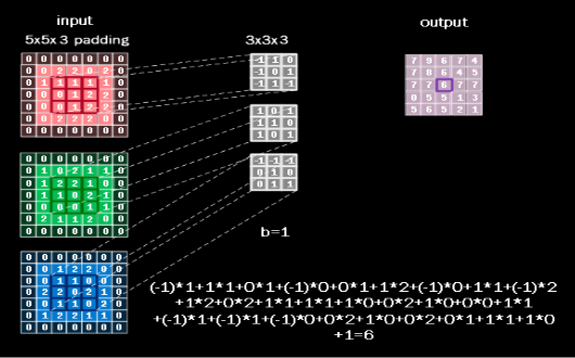
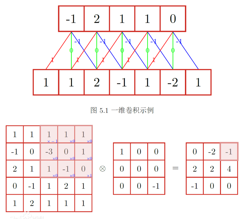
卷积是一种提取图片特征的方法,一般用一个正方形卷积核,遍历图片上的每一个像素点。图片与卷积内相对应的权重,然后求和,再加上偏置后,最后输出一个图片的像素值(图片来自网络,侵权请联系删除)。

tensorflow{:height=”600px” width=”600px”}

全零填充Padding

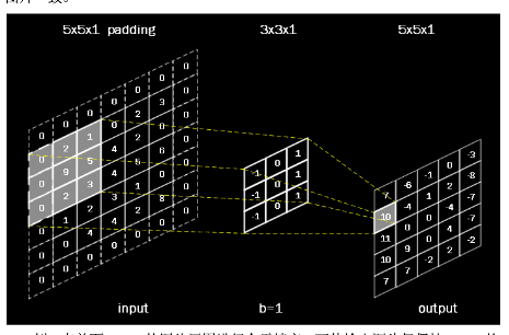
正常的卷积会导致图片的缩小,为了能够让输入和输出的图片尺寸一致,对图片周围的空数据进行全0填充。(图片来自网络,侵权请联系删除)。

tensorflow{:height=”600px” width=”600px”}

阅读全文 »

MINST数据库是由是一个手写数字的数据集,官方网址:http://yann.lecun.com/exdb/mnist/

 > MNIST 数据集来自美国国家标准与技术研究所, National Institute of Standards and Technology (NIST). 训练集 (training set) 由来自 250 个不同人手写的数字构成, 其中 50% 是高中学生, 50% 来自人口普查局 (the Census Bureau) 的工作人员. 测试集(test set) 也是同样比例的手写数字数据.

MINST数据总共有4个包,解压出来的数据如下:

tensorflow{:height=”600px” width=”600px”}

  1. train-images-idx3-ubyte.gz,train-labels-idx1-ubyte.gz:提供了60000张,28*28像素的黑底白字图片用来训练
  2. t10k-images-idx3-ubyte.gz,t10k-labels-idx1-ubyte.gz:提供了10000张,28*28像素的黑底白字图片用来测试

mnist提供的图片有784(28*28)个像素点,把每个像素点的值,组织成一个一维的数组,作为输入参数。形式如下:

1
2
3
4
5
6
7
8
9
10
11
12
13
14
15
16
17
18
19
20
21
22
23
24
25
26
27
28
29
30
31
32
33
34
35
36
37
38
39
40
41
42
43
44
45
46
47
48
49
50
51
52
53
54
55
56
 [0. 0. 0. 0. 0. 0. 0. 0. 0. 0. 0.386 0.379 0....... 0. 0. 0. 0. 0. 0. 0. 0. 0. 0. 0. ]
```

图片的标签以一维数组给出,每个元素代表出现的概率,形式如下:

`[0. 0. 0. 0. 0. 0. 1. 0. 0. 0. ]` 代表数字6


`tensorflow`官方支持数据集的读取,使用代码如下:

``` python
# coding:utf-8
from tensorflow.examples.tutorials.mnist import input_data

minst=input_data.read_data_sets('./data/',one_hot=True)
#打印数据数量
print( "train data size:",minst.train.num_examples)
print( "validation data size:",minst.validation.num_examples)
print( "test data size:",minst.test.num_examples)

#打印数据
print(minst.train.labels[0])
print(minst.train.images[0])

#打印前200行数据
BATCH_SIZE=200
xs,ys=minst.train.next_batch(BATCH_SIZE)
print("xs shape:",xs.shape)
print("ys shape:",ys.shape)

```

输出到控制台结果:

``` cte
train data size: 55000
validation data size: 5000
test data size: 10000
[0. 0. 0. 0. 0. 0. 0. 1. 0. 0.]
[ 0. 0.....0. 0.3529412 0.5411765 0.9215687 0.9215687 0.9215687 0.9215687 0.9215687 0.9215687 0.9843138 0.9843138 0.9725491 0.9960785 0.9607844 0.9215687 0.74509805 0.08235294 0. 0. 0.....]
xs: [[0. 0. 0. ... 0. 0. 0.]
[0. 0. 0. ... 0. 0. 0.]
[0. 0. 0. ... 0. 0. 0.]
...
[0. 0. 0. ... 0. 0. 0.]
[0. 0. 0. ... 0. 0. 0.]
[0. 0. 0. ... 0. 0. 0.]]
xs shape: (200, 784)
ys: [[0. 0. 0. ... 0. 0. 0.]
[0. 0. 0. ... 1. 0. 0.]
[0. 0. 0. ... 0. 0. 0.]
...
[0. 0. 0. ... 0. 0. 0.]
[0. 0. 1. ... 0. 0. 0.]
[1. 0. 0. ... 0. 0. 0.]]
ys shape: (200, 10)

既然是图片数据,我们就能把他们都还原过去,代码如下:

1
2
3
4
5
6
7
8
9
10
11
12
13
14
15
16
17
18
19
20
21
22
23
24
25
26
27
28
29
30
31
32
33
34
35
36
37
38
39
40
41
42
43
44
45
46
47
48
49
50
51
#coding:utf-8
import numpy as np
import struct

from PIL import Image
import os

data_file = 'train-images-idx3-ubyte' #需要修改的路径

# It's 47040016B, but we should set to 47040000B
data_file_size = 47040016
data_file_size = str(data_file_size - 16) + 'B'

data_buf = open(data_file, 'rb').read()

magic, numImages, numRows, numColumns = struct.unpack_from(
'>IIII', data_buf, 0)
datas = struct.unpack_from(
'>' + data_file_size, data_buf, struct.calcsize('>IIII'))
datas = np.array(datas).astype(np.uint8).reshape(
numImages, 1, numRows, numColumns)

label_file = 'train-labels-idx1-ubyte' #需要修改的路径

# It's 60008B, but we should set to 60000B
label_file_size = 60008
label_file_size = str(label_file_size - 8) + 'B'

label_buf = open(label_file, 'rb').read()

magic, numLabels = struct.unpack_from('>II', label_buf, 0)
labels = struct.unpack_from(
'>' + label_file_size, label_buf, struct.calcsize('>II'))
labels = np.array(labels).astype(np.int64)

datas_root = './pic/' #需要修改的路径
if not os.path.exists(datas_root):
os.mkdir(datas_root)

for i in range(10):
file_name = datas_root + os.sep + str(i)
if not os.path.exists(file_name):
os.mkdir(file_name)

for ii in range(numLabels):
img = Image.fromarray(datas[ii, 0, 0:28, 0:28])
label = labels[ii]
#不足5位补0版本
file_name = datas_root + os.sep + str(label) + os.sep + \
str(ii).zfill(5) + '.png'
img.save(file_name)

tensorflow

阅读全文 »

今天整理下学习的tensorflow的几个常用的方法和代码片段.

  1. tf.get_collection("") 从集合中取出全部变量,生成一个列表

  2. tf.add_n([]) 列表内对应元素相加

  3. tf.cast(x,dtype) 把x转为dtype类型

  4. tf.argmax(x,axis) 返回最大值所在索引号,如 tf.argmax([0,1,0]) 返回2

  5. with tf.Graph().as_default() as g: 其内定义的节点在计算图g中

  6. 保存模型:

    1
    2
    3
    4
    5
    6
    7
    8
    9
    10
    11
    12
    13
    14
    15
    16
            saver=tf.train.Saver()# 实例化saver对象
    with tf.Session() as sess: # 在with结构的for循环一定轮数是,保存模型到当前会话
    for i in range(STEPS):
    if i%轮数 ==0
    saver.save(sess,os.path.join(""),global_step=global_step)

    ```

    7. 加载模型

    ``` python

    with tf.Session() as sess:
    ckpt=tf.train.get_checkpoint_path
    if ckpt and ckpt.model_checkpoint_path:
    saver.restore(sess,ckpt.model_checkpoint_path)
  7. 反向传播均方误差和减少loss

    1
    2
    3
    4
    5
    loss=tf.reduce_mean(tf.square(y_-y))
    # 三个减少loss的训练方法
    train_step=tf.train.GradientDescentOptimizer(learnig_rate).minimize(loss)
    train_step=tf.train.MomentumOptimizer(learnig_rate,momentum).minimize(loss)
    train_step=tf.train.AdamOptimizer(learnig_rate).minimize(loss)
  8. 损失函数

    1
    2
    3
    4
    5
    6
    7
    # tf.nn.relu   #未找到使用地方
    # tf.nn.sigmoid #未找到使用地方
    # tf.nn.tanh #未找到使用地方
    loss=tf.reduce_sum(tf.where(tf.greater(y,y_),COST(y-y_),PROFIT(y_-y))) #自定义损失函数

    ce=tf.nn.sparse_softmax_cross_entropy_with_logits(logtis=y,labels=tf.argmax(y_,1))#交叉熵
    cem=tf.reduce_mean(ce)#交叉熵
  9. 学习率计算

    1
    2
    3
    4
    5

    # 指数衰减学习率
    global_step=tf.Variable(0,trainable=False)
    learning_rate=tf.train.exponential_decay(LEARNINF_RATE_BASE,global_step,LEARNINF_RATE_STEP,LEARNINF_RATE_DECAY,staircase=True)

  1. 滑动平均

    1
    2
    3
    4
    5
    6
    7
    8
    9
    10
    ema=tf.train.ExponentialMovingAverage(衰减率MOVING_AVERAGE_DECAY,当前轮数global_step)   

    ema_op=ema.apply([])
    ema_op=ema.apply(tf.trainable_variables()) # 每运行此据,所有待优化的参数求滑动平均

    with tf.control_dependencies([train_step,ema_op]):
    train_op=tf.no_op(name='train')

    ema.average(查看参数的滑动平均)

  2. 正则化

    1
    2
    3
    4
    5
    6
    loss(w)=tf.contrib.layers.l1_regularizer(REGULARIZER)(w) #w加和
    loss(w)=tf.contrib.layers.l2_regularizer(REGULARIZER)(w) # w平方加和

    tf.add_to_collection('losses',tf.contrib.layers.l2_regularizer(regularizer)(w))

    loss=cem+tf.add_n(tf.get_collection('losses'))
  3. 实例化可还原滑动平均值的saver

    1
    2
    3
    ema=tf.train.ExponentialMovingAverage(滑动平均数)
    ema_restore=ema.variable_to_restore()
    saver=tf.train.Saver(ema_restore)
  4. 准确率计算方法

    1
    2
    correct_prediction=tf.equal(tf.argmax(y,1),tf.argmax(y_,1))
    accuracy=tf.reduce_mean(tf.cast(correct_prediction,tf.float32))
阅读全文 »

这几天终于把tensorflow的基础学完了,虽然还有点云里雾里,但毕竟入门是一件困难的事情。下面把这几次的写的代码整理出来。

generateds.py文件

1
2
3
4
5
6
7
8
9
10
11
12
13
14
15
16
17
18
19
20
21
22
23
24
25
26
27
28
29
30
31
32
33
34
35
36
37
38
39
40
41
42
43
44
45
46
47
48
49
50
51
52
53
54
55
56
57
58
59
60
61
62
63
64
65
66
67
68
69
70
71
72
73
74
75
76
77
78
79
80
81
82
83
84
85
86
87
88
89
90
91
92
93
94
95
96
97
98
99
100
101
102
103
104
105
106
107
108
109
110
111
112
113
114
115
116
117
118
119
120
121
122
123
import numpy as np
import matplotlib.pyplot as plt

seed=2

def generateds():
# 基于seed产生随机数
rdm=np.random.RandomState(seed)
# 随机数返回300行2列的矩阵,表示300组坐标点
X=rdm.randn(300,2)

Y_=[int(x0*x0+x1*x1<2) for (x0,x1) in X]

# 遍历Y中的每个元素,1赋值'red',其余的赋值blue
Y_c=[['red' if y else 'blue' for y in Y_]]

# 对数据集X和标签Y进行形状的整理,第一个元素为-1 ,表示跟随第二列计算,第二个元素表示多少列,可见X为两列,Y为1列
X=np.vstack(X).reshape(-1,2)
Y_=np.vstack(Y_).reshape(-1,1)

return X,Y_,Y_c

if __name__=="__main__":
X,Y_,Y_c=generateds()
print("X:\n",X) # 300*2
print("Y_:\n",Y_)# 300*1
print("Y_c:\n",Y_c) # 1*300

```

`forward.py文件`
``` python
# coding:utf-8

import tensorflow as tf

def get_weight(shape,regularizer):
w=tf.Variable(tf.random_normal(shape),dtype=tf.float32)
tf.add_to_collection("losses",tf.contrib.layers.l2_regularizer(regularizer)(w))
return w

def get_bias(shape):
b=tf.Variable(tf.constant(0.01,shape=shape))
return b


def forward(x,regularizer):
w1=get_weight([2,11],0.01)
b1=get_bias([11])
y1=tf.nn.relu(tf.matmul(x,w1)+b1)

w2=get_weight([11,1],0.01)
b2=get_bias([1])
y=tf.matmul(y1,w2)+b2
return y

```

最终利用所有的方法拟合的代码:


``` python
# coding:utf-8

import tensorflow as tf
import numpy as np
import matplotlib.pyplot as plt
import generateds
import forward

STEPS = 40000
BATCH_SIZE = 30
LEARNING_RATE_BASE = 0.001
LEARNING_RATE_DECAY = 0.999
REGULARIZER = 0.01


def backward():
x = tf.placeholder(tf.float32, shape=(None, 2))
y_ = tf.placeholder(tf.float32, shape=(None, 1))

X, Y_, Y_c = generateds.generateds()
y = forward.forward(x, REGULARIZER)

global_step = tf.Variable(0, trainable=False)
learning_rate = tf.train.exponential_decay(LEARNING_RATE_BASE, global_step, 300 / BATCH_SIZE, LEARNING_RATE_DECAY,
staircase=True)

# 定义损失函数
loss_mse = tf.reduce_mean(tf.square(y - y_))


loss_total = loss_mse + tf.add_n(tf.get_collection('losses'))
# 定义反向传播方法:包含正则化
train_step = tf.train.AdadeltaOptimizer(learning_rate).minimize(loss_total)

with tf.Session() as sess:
init_op = tf.global_variables_initializer()
sess.run(init_op)

for i in range(STEPS):
start = (i * BATCH_SIZE) % 300
end = start + BATCH_SIZE
sess.run(train_step, feed_dict={x: X[start:end], y_: Y_[start:end]})

if i % 2000 == 0:
loss_v = sess.run(loss_total, feed_dict={x: X, y_: Y_})
print("After %d training steps,loss on all data is %f" % (i, loss_v))

xx, yy = np.mgrid[-3:3:0.01, -3:3:0.01]
grid = np.c_[xx.ravel(), yy.ravel()]
probs = sess.run(y, feed_dict={x: grid})
probs = probs.reshape(xx.shape)

plt.scatter(X[:, 0], X[:, 1], c=np.squeeze(Y_c))
plt.contour(xx, yy, probs, levels=[.5])
plt.show()


if __name__ == "__main__":
backward()


阅读全文 »