tensorflow的学习笔记--损失函数

损失函数

在前面几个博客中说了一个学习模型，具体表现如下：

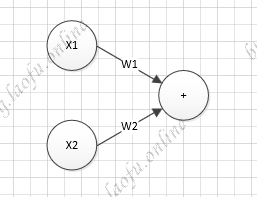
具体的计算公式：$$Y=\sum_{i}^nX_iW_i$$

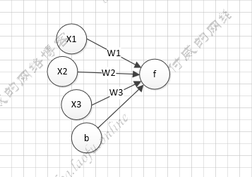
曾经有人提出另一个神经元模型，多了激活函数和偏执项。

具体的计算公式：
$$
Y=f(\sum_{i}^nX_iW_i+b)
$$
其中f是激活函数,b是偏执项。

损失函数（loss）：预测值y’和已知答案y的差距

我们的优化目标就是把loss降低为最小。

激活函数

引入激活函数有效的避免仅使用$$XW$$的线性组合，是模型更准确，更具有表达能力。

常用的激活函数有：

1. relu（tf.nn.relu）：
   $$
   f(x)=max(x,0)= \begin{cases}
   0, & \text{$x<=0$} \
   x, & \text{$x>0$}
   \end{cases}
   $$

   用tensorflow表示为:tf.nn.relu ,函数图像为：

​

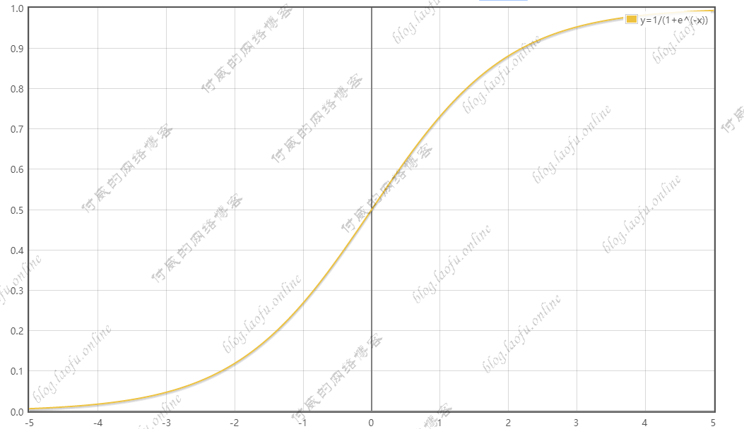
2. sigmoid（tf.nn.sigmoid）:
   $$
   f(x)=1/(1+e^x)
   $$
   用tensorflow表示为:tf.nn.sigmoid,函数图像为：

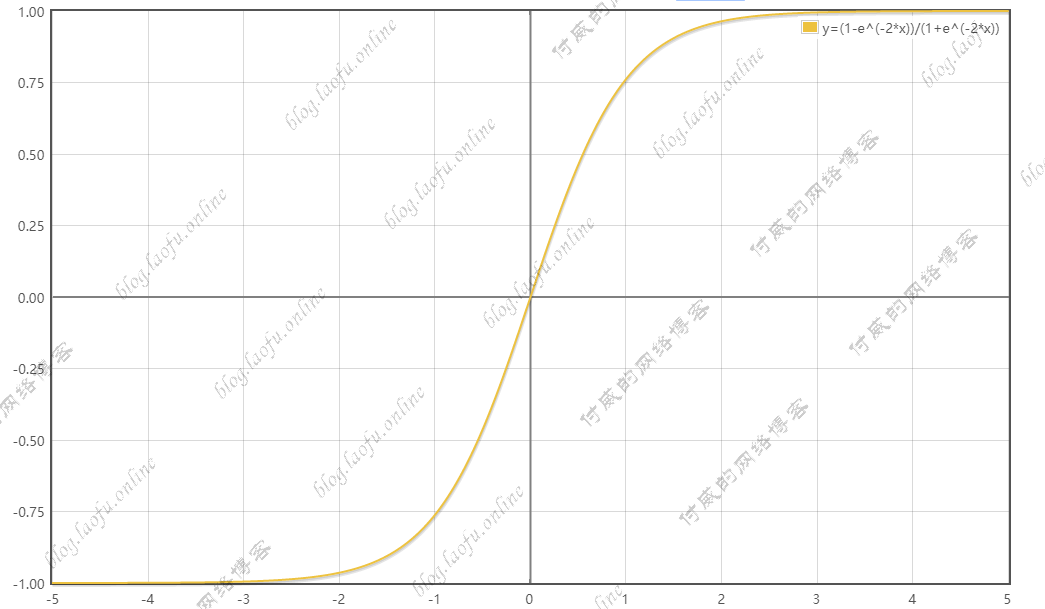
3. tanh:
   $$
   f(x)=(1-e^{-2x})/(1+e^{-2x})
   $$

   用tensorflow表示为:tf.nn.tanh,函数图像为：

举个例子

预测酸奶的日销量，x1、x2是影响日销量的因素，建模前应预先猜测的数据有：每日x1、x2和销量y_（即已知答案，最佳情况，产量=销量）拟造数据集X,Y;y_=x1+x2,噪声是-0.05~+0.05 拟合可以预测销量的函数。

根据上面的模型，我们生成随机数，进行训练，代码如下：

#coding:utf-8
import tensorflow as tf
import numpy as np
BATCH_SIZE=8
seed=23455


rdm=np.random.RandomState(seed)
X=rdm.rand(32,2)
Y_=[[x1+x2+(rdm.rand()/10.0-0.05)] for(x1,x2) in X]


#定义神经网络输入，参数和输出，定义前向传播  

x=tf.placeholder(tf.float32,shape=(None,2))
y_=tf.placeholder(tf.float32,shape=(None,1))
w1=tf.Variable(tf.random_normal([2,1],stddev=1,seed=1))
y=tf.matmul(x,w1)


#2 定义损失函数及反向传播方法
# 定义损失函数数MSE，方向传播方法为梯度下降   

loss_mse=tf.reduce_mean(tf.square(y_-y))
train_step=tf.train.GradientDescentOptimizer(0.001).minimize(loss_mse)

#生成会话，训练step

with tf.Session() as sess:
init_op=tf.global_variables_initializer()
sess.run(init_op)
STEPS=20000
for i in range(STEPS):
     start=(i*BATCH_SIZE)%32
     end =(i*BATCH_SIZE)%32+BATCH_SIZE
     sess.run(train_step,feed_dict={x:X[start:end],y_:Y_[start:end]})

     if i%500==0:
          print ("After %d training steps,wl isL" %(i))
          print (sess.run(w1))
print("final wl is:\n",sess.run(w1))

打印结果：

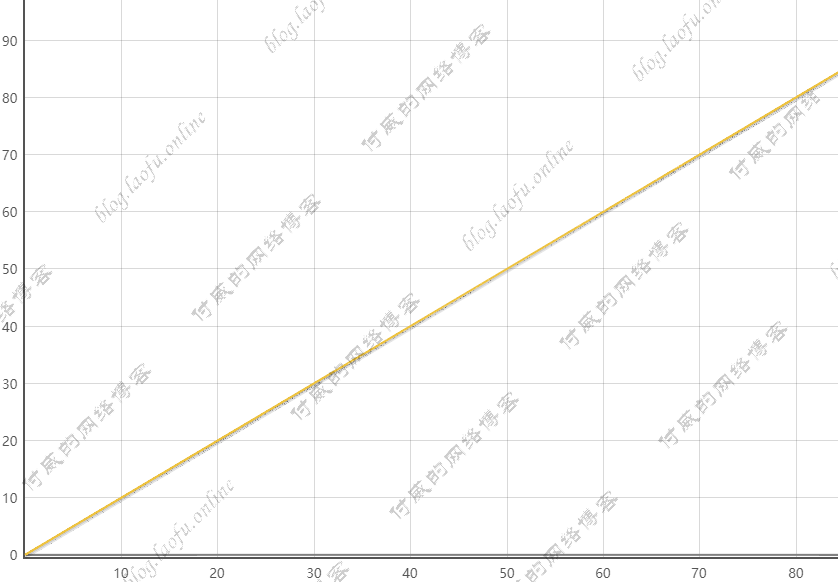
After 17500 training steps,wl isL
[[0.96476096]
[1.0295546 ]]
After 18000 training steps,wl isL
[[0.9684917]
[1.0262802]]
After 18500 training steps,wl isL
[[0.9718707]
[1.0233142]]
After 19000 training steps,wl isL
[[0.974931 ]
[1.0206276]]
After 19500 training steps,wl isL
[[0.9777026]
[1.0181949]]
final wl is:
[[0.98019385]
[1.0159807 ]]

看到两个权重的值，都趋于1. 与数据结果y=x1+x2 结果一致。

自定义损失函数

在预测商品销量，预测多了，损失成本，预测少了损失利润，若利润不等于成本，则mse产生的loss无法利益最大化。

自定义损失函数 $$\sum_{i}^nf(y’,y)$$

$$
f(y’,y) =
\begin{cases}
PROFIT*(y’-y), & \text{$y<y’$ 预测y少了，损失利润（PROFIT）} \
COST*(y-y’), & \text{$y>=y’$ 预测y多了，损失成本（COST）}
\end{cases}
$$

使用下面的函数进行修正： loss=tf.reduce_sum(tf.where(tf.greater(y,y_),COST(y-y_),PROFIT(y_-y)))

如上面的例子，酸奶的成本（COST)1元，酸奶的利润（PROFIT)9元。
预测少了损失利润9元，预测多了损失成本预测。

预测少了损失大，希望生成的预测函数。往多了预测。

我们把损失函数进行替换，换成我们的自定义的函数，代码如下：

#coding:utf-8
#预测少了损失利润9元，预测多了损失成本预测。  
import tensorflow as tf
import numpy as np
BATCH_SIZE=8
seed=23455
COST=1
PROFIT=9


rdm=np.random.RandomState(seed)
X=rdm.rand(32,2)
Y_=[[x1+x2+(rdm.rand()/10.0-0.05)] for(x1,x2) in X]


#定义神经网络输入，参数和输出，定义前向传播  

x=tf.placeholder(tf.float32,shape=(None,2))
y_=tf.placeholder(tf.float32,shape=(None,1))
w1=tf.Variable(tf.random_normal([2,1],stddev=1,seed=1))
y=tf.matmul(x,w1)


#2 定义损失函数及反向传播方法
# 定义损失函数数MSE，方向传播方法为梯度下降   

# loss_mse=tf.reduce_mean(tf.square(y_-y))
loss_mse=tf.reduce_sum(tf.where(tf.greater(y,y_),COST*(y-y_),PROFIT*(y_-y)))
train_step=tf.train.GradientDescentOptimizer(0.001).minimize(loss_mse)

#生成会话，训练step

with tf.Session() as sess:
init_op=tf.global_variables_initializer()
sess.run(init_op)
STEPS=20000
for i in range(STEPS):
     start=(i*BATCH_SIZE)%32
     end =(i*BATCH_SIZE)%32+BATCH_SIZE
     sess.run(train_step,feed_dict={x:X[start:end],y_:Y_[start:end]})

     if i%500==0:
          print ("After %d training steps,wl isL" %(i))
          print (sess.run(w1))
print("final wl is:\n",sess.run(w1))

After 18500 training steps,wl isL
[[1.0232253]
[1.0445153]]
After 19000 training steps,wl isL
[[1.0171654]
[1.038825 ]]
After 19500 training steps,wl isL
[[1.0208615]
[1.0454264]]
final wl is:
[[1.020171 ]
[1.0425103]]

可以看到预测尽量往多的方向去预测。

交叉熵

交叉熵表示两个概率分布之间的距离。

$$
H(y’,y)=-\sum y’*logy
$$

例如，已知答案y’=(1,0),预测**y1=(0.6,0.4) y2=(0.8,0.2)**哪个更接近标准答案？

$$
H_1((1,0),(0.6,0.4))=-(1log0.6+0log0.4)\approx0.222
$$

$$
H_2((1,0),(0.8,0.2))=-(1log0.8+0log0.2)\approx0.097
$$

所以y2预测更为准确。

我们可以使用交叉熵的形式，来更精确的训练我们的模型。

ce=-tf.reduce_mean(y'*tf.log(tf.clip_by_value(y,1e^-12,1.0)))

其中y<1e^-12是，y=1e^-12，防止log0的出现

当n分类的n个输出（y1,y2,…yn）通过softmax()函数,便满足了概率的分布要求：

$$
P(X=x)\rightarrow[0,1] 且 \sum P(X=x)=1
$$

$$
softmax(y_i)=\frac{e^{y_i}}{\sum_{j=1}^ne^{y_i}}
$$
可以用ce=tf.nn.sparse_softmax_cross_entropy_with_logits(logtis=y,labels=tf.argmax(y_,1))

cem=tf.reduce_mean(ce) 替换交叉熵的函数，代表的是当前的预测值与标准答案的差距。

​