一以贯之搭建神经网络的过程
在神经网络中预测识别和预测的过程中,其实都是一个函数的对应关系: 的函数关系,为了找到这个函数的关系,我们需要做大量的训练,具体的过程可以总结下面几个步骤:
获得随机矩阵w1和b1,经过一个激活函数,得到隐藏层。
获得随机矩阵w2和b2,计算出对应的预测y
利用y与样本y_的差距,有平方差和交叉熵等方式,来定义损失函数
利用指数衰减学习率,计算出学习率
用滑动平均计算输出的参数的平均值
利用梯度下降的方法,减少损失函数的差距
用with结构初始化所有的参数
利用for循环喂入数据,反复训练模型
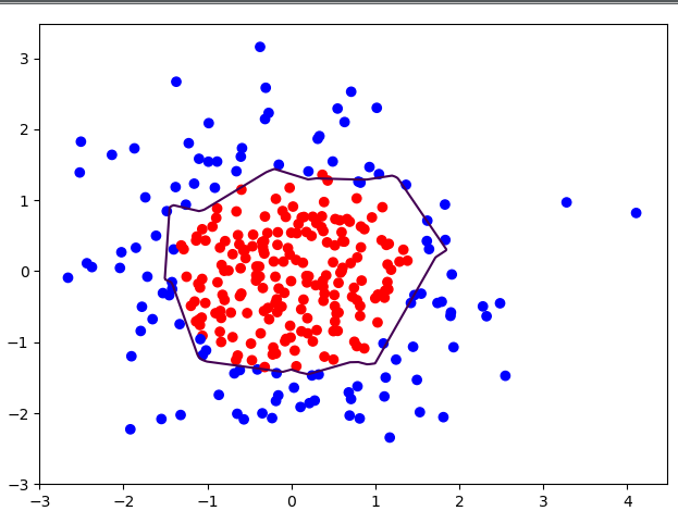
利用这个八个步骤拟合出的一个圆的函数,代码和结果如下:
1
2
3
4
5
6
7
8
9
10
11
12
13
14
15
16
17
18
19
20
21
22
23
24
25
26
27
28
29
30
31
32
33
34
35
36
37
38
39
40
41
42
43
44
45
46
47
48
49
50
51
52
53
54
55
56
57
58
59
60
61
62
63
64
65
66
67
68
69
70
71
72
73
74
75
76
77
78
79
80
81
82
83
84
85
86
87
88
89
90
91
92
93
94
95
96
97
98
99
100
101
102
103
104
105
106
107
108
109
110
111
112
113
114
115
116
# coding:utf-8
import os
import tensorflow as tf
import numpy as np
import matplotlib.pyplot as plt
xLine = 300
aLine = 10
BATCHSIZE = 10
regularizer=0.001
BASE_LEARN_RATE=0.001
LEARNING_RATE_DECAY = 0.99
MOVING_VERAGE_DECAY=0.99
# 1 生成随机矩阵x
rdm = np.random.RandomState(2)
X = rdm.randn(xLine, 2)
print("1.生成X:", X)
# 2 生成结果集Y
Y = [int(x1 * x1 + x2 * x2 < 2) for (x1, x2) in X]
print("2.生成Y:", Y)
Y_c = [['red' if y else 'blue'] for y in Y]
print("3. 生成Y_c:", Y_c)
X = np.vstack(X).reshape(-1, 2)
Y = np.vstack(Y).reshape(-1, 1)
print("4. 生成X:", X)
print("5. 生成Y:", Y)
# plt.scatter(X[:, 0], X[:, 1], c=np.squeeze(Y_c))
# plt.show()
# 3. 这里如何保存数据集为样本?
# 4. 训练样本占位
x = tf.placeholder(tf.float32, shape=(None, 2))
y_ = tf.placeholder(tf.float32, shape=(None, 1))
global_step=tf.Variable(0,trainable=False)
# 5. 获得随机矩阵w1和b1,计算隐藏层a
w1 = tf.Variable(tf.random_normal(shape=([2, aLine]))) # 2*100
tf.add_to_collection("losses",tf.contrib.layers.l2_regularizer(regularizer)(w1))
b1 =tf.Variable(tf.constant(0.01, shape=[aLine])) # 3000*100
# 6.使用激活函数计算隐藏层a
a = tf.nn.relu(tf.matmul(x, w1) + b1) # 3000*2 x 2*100 +3000*100
# 7. 获得随机矩阵w2和b2 计算预测值y。
w2 = tf.Variable(tf.random_normal(shape=([aLine, 1])))
tf.add_to_collection("losses",tf.contrib.layers.l2_regularizer(regularizer)(w2))
b2 = tf.Variable(tf.random_normal(shape=([1])))
y = tf.matmul(a, w2) + b2
# 8. 损失函数
loss = tf.reduce_mean(tf.square(y - y_))
# loss = tf.reduce_mean(tf.square(y - y_))
# 滑动学习率
learning_rate=tf.train.exponential_decay(BASE_LEARN_RATE,
global_step,
BATCHSIZE,
LEARNING_RATE_DECAY,
staircase=True)
# 9. 梯度下降方法训练
train_step = tf.train.GradientDescentOptimizer(0.001).minimize(loss)
# 滑动平均
# ema=tf.train.ExponentialMovingAverage(MOVING_VERAGE_DECAY,global_step)
# ema_op=ema.apply(tf.trainable_variables())
# with tf.control_dependencies([train_step,ema_op]):
# train_op=tf.no_op(name="train")
saver=tf.train.Saver()
# 10. 开始训练
with tf.Session() as sess:
init_op = tf.global_variables_initializer()
sess.run(init_op)
STEPS = 40000
for i in range(STEPS):
start = (i * BATCHSIZE) % xLine
end = start + BATCHSIZE
# print(Y[start:end])
sess.run(train_step, feed_dict={
x: X[start:end],
y_: Y[start:end]
})
if i % 2000 == 0:
# learning_rate_val=sess.run(learning_rate)
# print("learning_rate_val:",learning_rate_val)
loss_mse_v = sess.run(loss, feed_dict={x: X, y_: Y})
print("After %d training steps,loss on all data is %s" % (i, loss_mse_v))
saver.save(sess,os.path.join("./model/","model.ckpt"))
# print(global_step)
xx, yy = np.mgrid[-3:3:0.1, -3:3:.01]
grid = np.c_[xx.ravel(), yy.ravel()]
probs = sess.run(y, feed_dict={x: grid})
probs = probs.reshape(xx.shape)
print("w1:", sess.run(w1))
print("b1:", sess.run(b1))
print("w2:", sess.run(w2))
print("b2:", sess.run(b2))
plt.scatter(X[:, 0], X[:, 1], c=np.squeeze(Y_c))
plt.contour(xx, yy, probs, levels=[.5])
plt.show()